On double descent and complexity

Table of Contents
The story
A few years ago I made this poster for a course I took with [0]. There I decided to use compression as a proxy for the complexity of a ML model. I think I got the idea from [1].
The task here was to learn an image using some fancy spectral features and a linear model, and we observed the double descent phenomenon, for the over-parameterized regime we selected the minimum l2 norm solution for the model.
Risks
A little brush up on terminology:
Empirical Risk ($\hat R_n(h)$): The training error. It is the average loss over the $n$ samples used for training:
$$\hat R_n(h)=\frac{1}{n}\sum_{i=1}^n \ell(h(x_i),y_i)$$True Risk ($R(h)$): The generalization error (expected loss) over the full distribution $D$. We approximate this using the test error.:
$$R(h)= \mathbb{E}_{(x,y) \sim D}[\ell(h(x),y)]$$
Double Descent
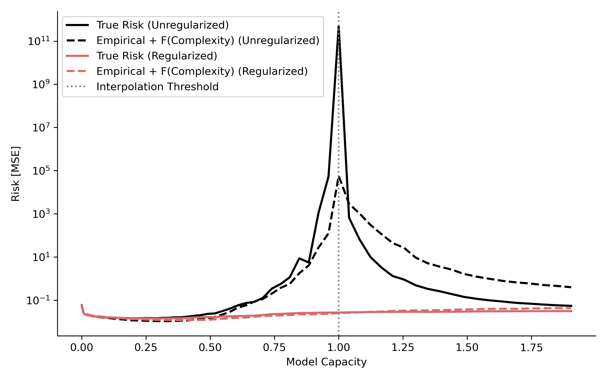
These are the two graphs I made back then:
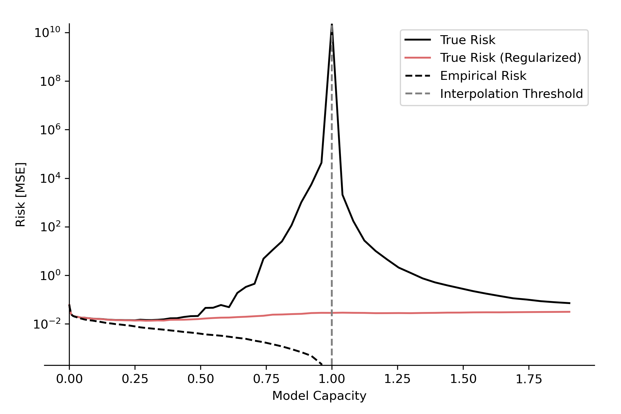
Empirical and true risk versus model capacity, illustrating the double descent phenomenon in our problem.
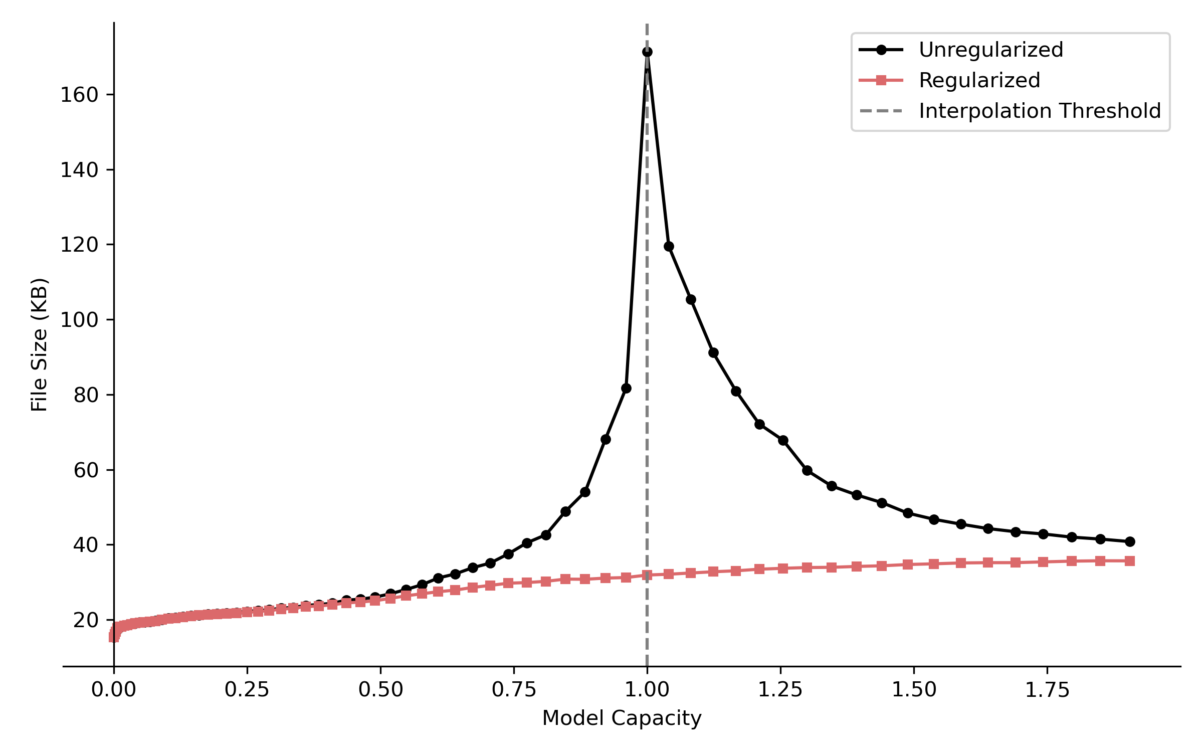
Compression versus model capacity showing the relationship between model size (as file size of the learned image) and number of parameters. This experiment was the first one to contradict my intuition that the larger the model, the more complex it would be.
What I did not notice at the time was how closely related my two graphs were; if I subtracted the empirical risk from the true risk, I obtained something very similar to the compression graph.
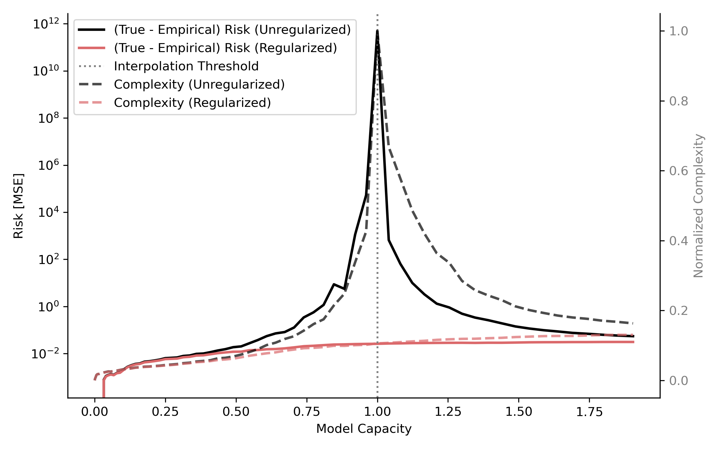
(true - empirical) risk and complexity versus model capacity.
Generalization
I later found [2], which analyzes double descent from the perspective of compression and provides bounds that relate true risk to compression. This video [3] by Ilya also touches on this point.
Fitting a power law merging risk vs. capacity graphs by capacity yields something like:
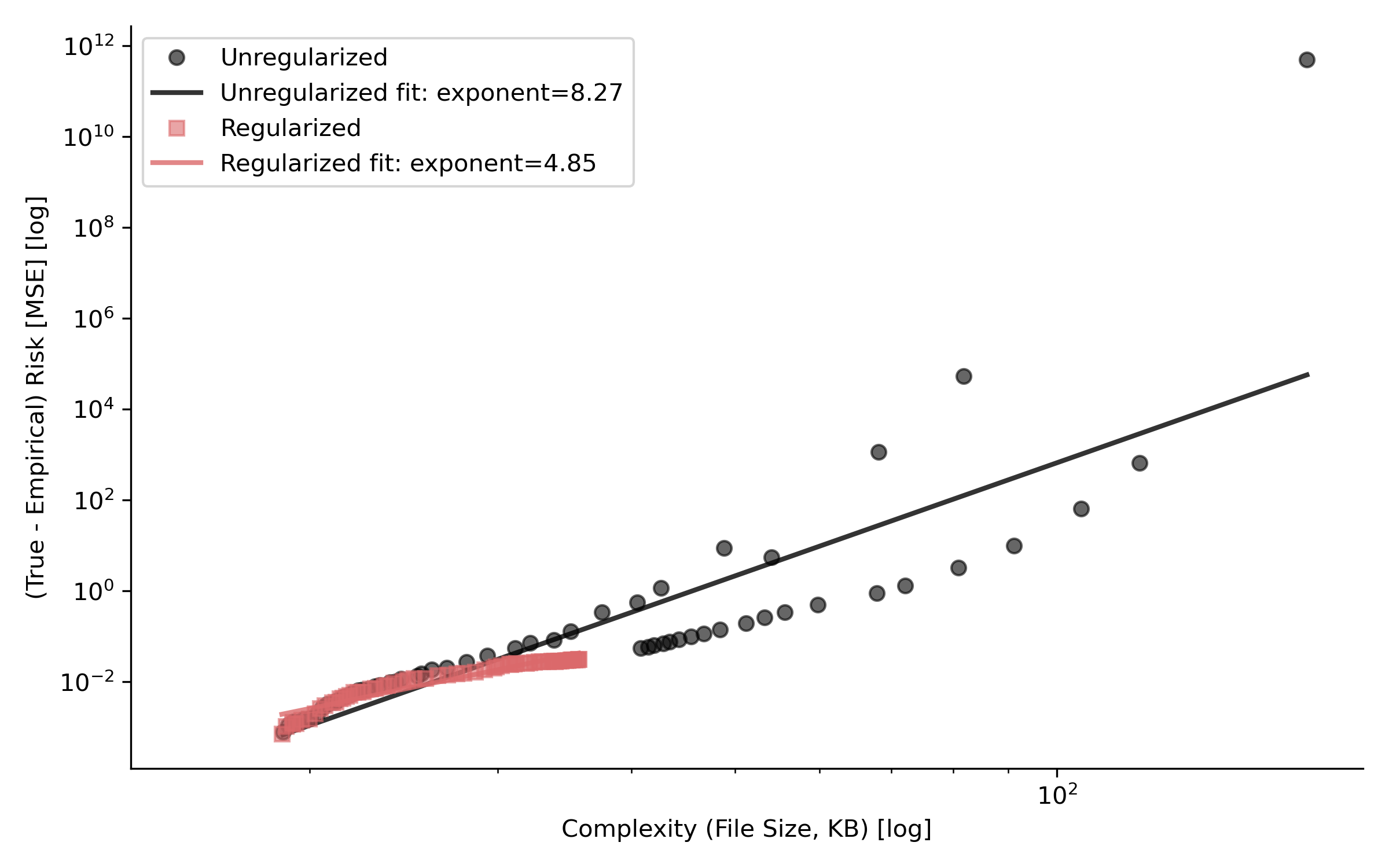
Power law fit to compression versus capacity data, showing the $\text{(True - Empirical) Risk} = \alpha \cdot \text{Complexity}^\beta$ relationship
Using this power law, I can somewhat predict generalization, which is interesting in itself.
True risk using the predictive compression-based power law relationship.
Bounds
Traditional PAC bounds tell us that if some reasonable hypotheses are true, then, with probability at least $1 - \delta$,
$$ R(h) \le \hat R_n(h) + \sqrt{\frac{\log \frac{1}{P(h)} + \log \frac{1}{\delta}}{2n}}. $$We can use a Solomonoff prior for $P(h) = 2^{-K(h|A)}$, where $K(h|A)$ is the Kolmogorov complexity.
What we are doing here is applying Occam’s razor (The simplest explanation is usually the best one) mathematically. This leaves us with:
$$R(h) \le \hat R_n(h) + \sqrt{\frac{K(h|A) + \log \frac{1}{\delta}}{2n}}.$$The meaning of this, roughly, is that the generalization error is bounded by the training error plus a term that depends on the complexity of the model, if the number of samples remains constant.
I’m loosely borrowing from [2] and [4] so please check them out for more details.
Is the Solomonoff prior always a good inductive bias?
Not always, the Data Generating Process is king after all, but in the absence of other information, Occam’s razor sounds like a reasonable assumption. Nature tends to favor simplicity.
A little aside, the Kolmogorov complexity is incomputable, but we can approximate it with compression, that’s how we tie all this together.
Are codecs good ML models then?
No.
What is not so surprising is that JPEG is good at compressing natural images. Codecs are highly optimized for their domains (image, video, audio), so they are naturally good compressors. But they are no good for ML mainly because they are not differentiable in several places.
The Huffman coding is not differentiable and handles much of the structural compression. You could use the DCT for feature extraction, and while quantizing DCT coefficients acts as a sort of $L_0$ regularization, forcing simplicity, it is also not differentiable. The color space transform is just a base change, totally learnable, so it does not make sense to use it as-is.
Codecs in general are not good models because they evolved via artificial selection for a related but different task, they only “train” on the test set.
References
[0] https://mate.dm.uba.ar/~pgroisma/
[1] D. Teney, A. Nicolicioiu, V. Hartmann, and E. Abbasnejad, “Neural Redshift: Random Networks are not Random Functions,” arXiv preprint arXiv:2403.02241, 2024.
[2] A. G. Wilson, “Deep Learning is Not So Mysterious or Different,” arXiv preprint arXiv:2503.02113, 2025.
[3] I. Sutskever, “An Observation on Generalization,” presented at Sequoia Capital AI Ascent 2024. https://www.youtube.com/watch?v=AKMuA_TVz3A
[4] P. Alquier, “User-friendly introduction to PAC-Bayes bounds,” arXiv preprint arXiv:2110.11216, 2021.